实战：利用决策树对波士顿房价数据集进行预测（附源码）

2023-10-27 14:49| 来源: 网络整理| 查看: 265

利用决策树对波士顿房价数据集进行预测

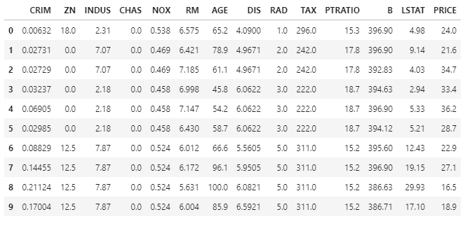
大家好，我是老马的程序人生~

使用sklearn提供的决策树（DecisionTreeRegressor）和线性回归（LinearRegression）的API对波士顿房价数据集进行预测，并尝试将预测结果进行分析。

1. 导入库 from sklearn.datasets import load_boston from sklearn.model_selection import cross_val_score from sklearn.tree import DecisionTreeRegressor from sklearn.linear_model import LinearRegression import pandas as pd import matplotlib.pyplot as plt 2. 加载数据

波士顿房价数据集来源于1978年美国某经济学杂志。

boston = load_boston() X = boston.data y = boston.target feature_names = boston.feature_names print(X.shape) # (506, 13) print(feature_names) # ['CRIM' 'ZN' 'INDUS' 'CHAS' 'NOX' 'RM' 'AGE' 'DIS' 'RAD' 'TAX' 'PTRATIO' 'B' 'LSTAT'] df = pd.DataFrame(X, columns=feature_names) df['PRICE'] = y print(df.head(10))

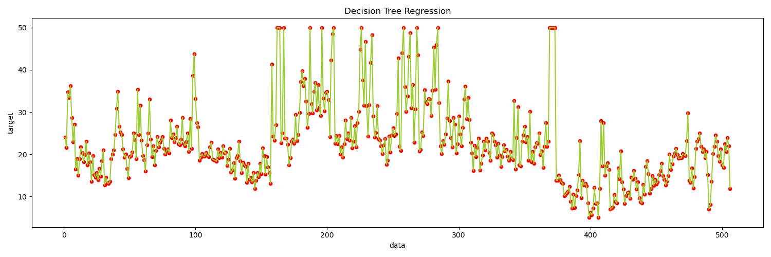
这些数据于1978年开始统计，共506个数据点，涵盖了麻省波士顿不同郊区房屋13种特征的信息，根据这些特征拟合房价。

特征：

CRIM：per capita crime rate by town 每个城镇人均犯罪率ZN：proportion of residential land zoned for lots over 25,000 sq.ft. 占地面积超过25,000平方英尺的住宅用地比例INDUS：proportion of non-retail business acres per town 非零售商用地百分比CHAS：Charles River dummy variable（= 1 if tract bounds river; 0 otherwise）是否靠近查尔斯河NOX：nitric oxides concentration (parts per 10 million) 氮氧化物浓度RM: average number of rooms per dwelling 住宅平均房间数目AGE：proportion of owner-occupied units built prior to 1940 1940年前建成自用单位比例DIS：weighted distances to five Boston employment centres 到5个波士顿就业服务中心的加权距离RAD：index of accessibility to radial highways 无障碍径向高速公路指数TAX：full-value property-tax rate per $10,000 每万元物业税率PTRATIO：pupil-teacher ratio by town 小学师生比例B：1000(Bk - 0.63)^2 where Bk is the proportion of blacks by town 黑人比例指数LSTAT: % lower status of the population 下层经济阶层比例

目标：

MEDV：Median value of owner-occupied homes in $1000’s 自有住房的中位数报价, 单位1000美元 3. 决策树 regressor = DecisionTreeRegressor(random_state=0) regressor = regressor.fit(X, y) y_pre = regressor.predict(X) plt.figure(figsize=(15, 5)) plt.scatter(range(1, 507), y, s=20, c='red') plt.plot(range(1, 507), y_pre, color='yellowgreen') plt.xlabel('data') plt.ylabel('target') plt.title('Decision Tree Regression') plt.show()

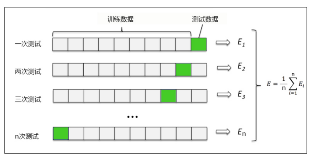
# 交叉验证cross_val_score的用法 cvs = cross_val_score(regressor , X , y , cv=10 , scoring='neg_mean_squared_error' ) print(cvs.mean()) # -33.91675098039215

交叉验证是用来观察模型的稳定性的一种方法，我们将数据划分为 n n n份，依次使用其中一份作为测试集，其他 n − 1 n-1 n−1份作为训练集，多次计算模型的精确性来评估模型的平均准确程度。训练集和测试集的划分会干扰模型的结果，因此用交叉验证 n n n次的结果求出的平均值，是对模型效果的一个更好的度量。

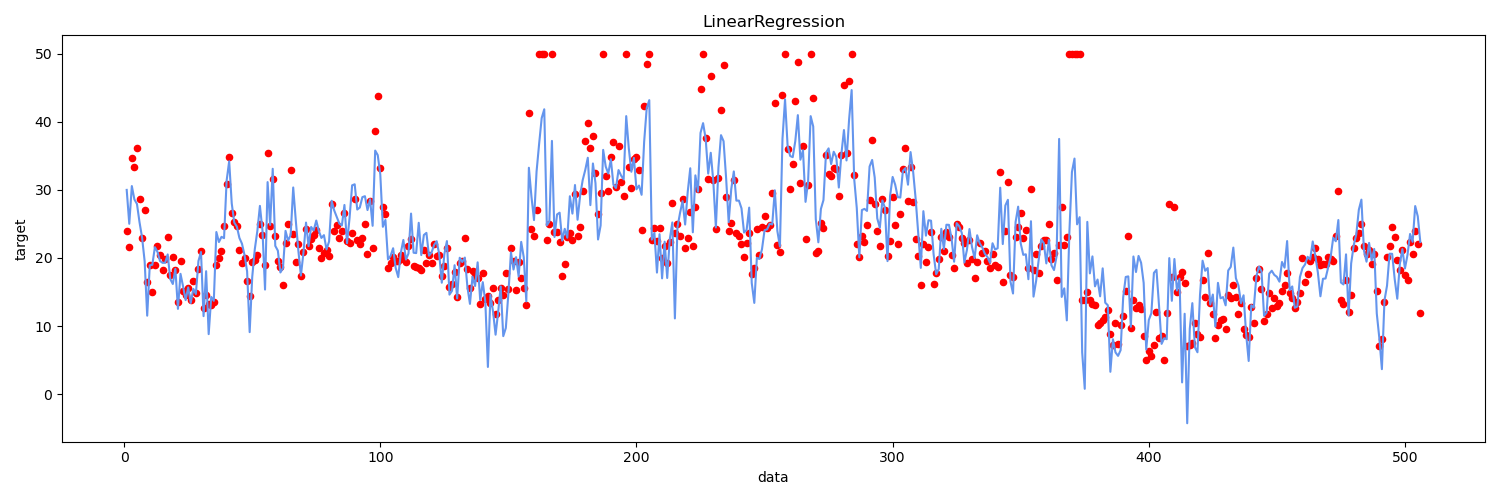
4. 线性回归 regressor = LinearRegression() regressor = regressor.fit(X, y) y_pre = regressor.predict(X) plt.figure(figsize=(15, 5)) plt.scatter(range(1, 507), y, s=20, c='red') plt.plot(range(1, 507), y_pre, color='cornflowerblue') plt.xlabel('data') plt.ylabel('target') plt.title('LinearRegression') plt.show()

# 交叉验证cross_val_score的用法 cvs = cross_val_score(regressor , X , y , cv=10 , scoring='neg_mean_squared_error' ) print(cvs.mean()) # -34.705255944524815 5. 分析

经过10次交叉验证，我们发现决策树的MSE为33.92，线性回归的MSE为34.71，决策树比线性回归的预测效果略好。

【本文地址】

公司简介

联系我们